K-Means Clustering using RStudio

Assalamualaikum Wr. Wb.

Hi data enthusiast!

On this occasion, we will learn about K-Means Clustering using the R Studio application. Actually, do you know about K-Means Clustering?

K-Means is a non-hierarchical data clustering method that seeks to partition existing data into one or more clusters or groups so that data with the same characteristics are grouped into the same cluster and data with different characteristics are grouped into clusters. the other group. K-Means is a distance-based clustering method that divides data into a number of clusters and this algorithm only works on numeric attributes. The K-Means algorithm includes partitioning clustering which separates data into separate sub-regions. The K-Means algorithm is very well known for its ease and ability to cluster large data and outlier data very quickly.

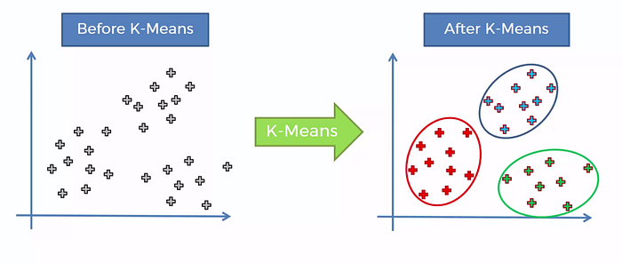
The stages in performing K-Means Clustering are as follows:

1. Determine the number of clusters
2. Allocate data into clusters randomly
3. Calculate the centroid/average of the data in each cluster
4. Allocate each data to the nearest centroid/average
5. Back to step 3, if there is still data moving clusters or if the centroid value changes, some are above the specified threshold value or if the change in the value in the objective function used is above the specified threshold value

Okeyy. let’s start! The data used this time is the Percentage of Villages/Urbans Based on Crime Incidents in Indonesia in 2018. The data is taken from village potential statistics (podes) 2018 records (bps.go.id)

The first step is to open RStudio, then input data.

data=read.delim("clipboard")
View(data)

Next, rename the variable to index.

index=data[,c(3:8)]
head(index)

Activate several packages that will be used. If you don’t have the package, install it first.

library(MVN)
library(PerformanceAnalytics)
library(factoextra)
library(ggubr)

Next, check the outlier data using the quan method.

outlier=,vn(index,multivariateOutlierMethod="quan",
            showNewData = TRUE)
chart.Correlation(index)

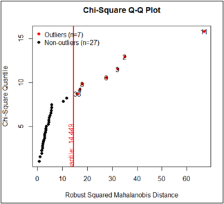
Based on the output, it can be seen that there are 7 provinces outliers, while the other 27 provinces are not outliers. However, this time we still use all observations and ignore data outliers.

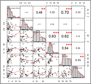
Based on the output, it can be seen that the correlation between variables is more dominant with low values, such as the correlation value of the X1 and X2 variables of 0.098, the correlation of X2 with X3 of 0.074, and other pairs of variables that have a low correlation. However, there is a fairly high correlation value of variables, namely the X1 and X5 variables, which are 0.7 and other pairs of variables that have a fairly high correlation. Pairs of variables that have low correlation values ​​result in the occurrence of symptoms of no multicollinearity or there is no relationship between the two variables (assuminganalysis is cluster non-hierarchicalmet).

Next, standardize the data as the first step in analyzing K-Means Clustering followed by calculating the distance between observations.

data_standarisasi=scale(index)
data_standarisasi
kluster=data_standarisasi
kluster
jarak=get_dist(kluster)
fviz_dist(jarak,gradient=list(low="#00AFBB",mid="white",high="#FC4                   E07"))

Based on the output, it can be seen that several provinces that have close proximity based on considerable distances are indicated by a darker orange color, and close proximity relationships are shown in blue, while white color indicates a measure of proximity based on medium distances.

The next step is to form clusters and create data frames resulting from the grouping.

k3=kmeans(kluster,centers=3,nstart=25)
k3
fviz_cluster(k3,data=kluster)
hasil=data.frame(index,k3$cluster)
hasil

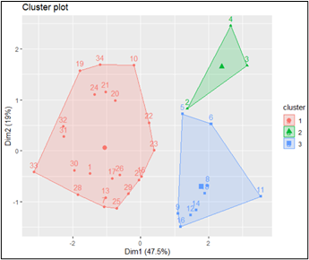
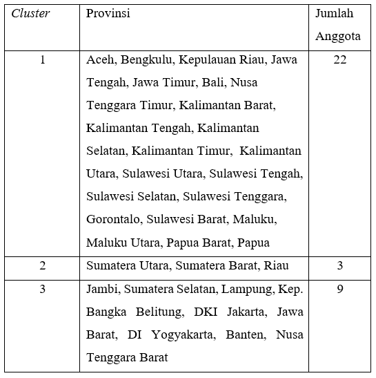
Based on the output in the form of clustering results, it can be seen that the results of grouping with 3 clusters standardizedhave better visualization than before because there is no buildup between clusters. In the output, it can be seen that the red area is cluster 1, cluster 2 is green and cluster 3 is blue.

For more details can be seen in the following table.

The last step is to identify the characteristics of each group.

kluster1=subset(hasil,k3,cluster==1)
kluster2=subset(hasil,k3,cluster==2)
kluster3=subset(hasil,k3,cluster==3)
kluster_1=sapply(kluster1,mean)
kluster_2=sapply(kluster2,mean)
kluster_3=sapply(kluster3,mean)
mean_total=rbind(kluster_1,kluster_2,kluster_3)
mean_total

The following characteristics are generated.

1. Cluster 1 is a provincial group that has a low percentage of theft with violence (X1), intentional arson (X2), drug abuse or dealers (X3), gambling (X4), theft (X5) and maltreatment (X6), while the percentage of arson with intentionally (X2) moderate.
2. Cluster 2 is a provincial group that has a moderate percentage of theft with violence (X1), theft (X5) and maltreatment (X6), while the percentage of intentional burning (X2), drug abuse or dealers (X3), gambling (X4) is high.
3. Cluster 3 is a provincial group that has a high percentage of violent theft (X1), theft (X5) and maltreatment (X6), while the percentage of drug dealers (X3), gambling (X4) is moderate, and the percentage of intentional arson (X2) is low.

That’s all i can explain, Thankyou and Have a Nice Day!:)

Wassalamualaikum Wr. Wb.